Vector Autoregression (VAR) of Longitudinal Sleep and Self-report Mood Data

This is an exploratory N-of-1 analysis involving four years of my own sleep data captured via the Oura Ring, a consumer-grade sleep tracking device, and my self-reported mood data logged via eMood Tracker for iOS. After assessing the data for stationarity and computing the appropriate lag-length selection, I fit a vector autoregressive (VAR) model and performed Granger causality tests to assess causal mechanisms within this multivariate time series. Oura’s nightly sleep quality score was shown to Granger-cause presence of depressed and anxious moods using a VAR(2) model.

Introduction

Long-term self-management of chronic illnesses such as bipolar disorder require persistent awareness of illness state over long periods of time and at varying time scales . Remaining consistently aware of key indicators signaling the onset of a chronic condition allow individuals a chance at early intervention to reduce the severity of a given episode. For example, an individual may modify behavior, engage their health practitioners, or adjust medication dosage. Bipolar disorder is an illness that often degrades an individual’s self-awareness and capacity for self-monitoring during symptomatic periods.

In the context of this specific illness, a volume of prior work has demonstrated the vital role of sleep in order to promote mood stability and prevent symptomatic episodes . Although the particulars of this topic fall beyond the scope of this paper, these nuanced relationships may in fact be self-reinforcing and bidirectional — poor sleep may lead to episodic onset, which may also lead to worsening (or shortening) sleep bouts.

Given the importance of sleep in the ongoing management of this illness, accurate consumer-grade alternatives to polysomnography (considered the gold standard of sleep tracking) have emerged over the last few years. Comparatively inexpensive sleep tracking technologies like the Oura Ring have dramatically improved the quality of information that can inform these self-monitoring activities. Objective sensor-based tracking technology can be complemented with subjective self-report measures in order to form a more complete picture of physical and mental health across time. Given the aforementioned interplay of sleep and mood, this combination of subjective and objective tracking creates the possibility of longitudinal analysis — and potentially deepens one’s capacity for self-awareness.

Following four years of consistent sleep and mood tracking, I wanted to interpret the data I had collected to quantify what I had intuited: that certain mood states could be understood (and potentially even predicted) by recent sleep trends. This intuition has been demonstrated quantitatively in existing literature .

I describe the methods used to achieve these goals, providing an overview of vector autoregression, Granger causality, and impulse response functions. I will detail the findings of these methods on the dataset, then conclude with a discussion of the methods and their potential applications in future work.

Methods

Problem setup

A multivariate time series analysis was performed using a vector autoregressive (VAR) model fit using ordinary least squares. An optimal lag order was first obtained using a combination of Akaike Information Criterion (AIC), Bayesian Information Criterion (BIC), Hannan-Quinn Information Criterion (HQIC), and final prediction error (FPE). After fitting a VAR(2) model on the multiple time series data (described below), a Granger causality test was performed in order to assess the predictive relationships between variables. Finally, an impulse response analysis was plotted to further explore the temporal relationships between variables, specifically between sleep and self-reported mood. I outline these analysis steps in greater detail in the sections that follow.

Vector Autoregression

A VAR($p$) model for a multivariate time series is a regression model for outcomes at time $t$ and time lagged predictors, with $p$ indicating the lag. Given $p$ = 1, the model would be concerned with one observation prior to $t$. A $T \times K$ multivariate time series (where $T$ is the number of observations and $K$ is the number of variables) can be modeled using a $p$-lag VAR model , notated as

\[Y_t = \nu + A_1 Y_{t-1} + \ldots + A_p Y_{t-p} + u_t\] \[u_t \sim {\sf Normal}(0, \Sigma_u)\]

where $A_i$ is a $K \times K$ coefficient matrix.

Intercept terms are included in $\nu$ and regression coefficients are included as the subscripted $A$ values. This equation is solved using ordinary least squares (OLS) estimation. The vector autoregressive (VAR) model is a flexible method for the analysis of causality in this setting.

Granger Causality Testing

I incorporated Granger causality tests to better assess the predictive capacity of the Oura sleep score on self-reported mood states. Granger causality defines one type of relationship between time series and states that a variable Granger causes another variable if “the prediction of one time series is improved by incorporating the knowledge of a second time series” .

Two autoregressive models are fit to the first time series, once with and once without the inclusion of the second time series. The improvement of the prediction is measured as the ratio of variance of the error terms. The null hypothesis states that the first variable does not Granger cause the second variable and is rejected if the coefficients for the lagged values of the first variable are significant.

In this study, Granger causation tests were applied using sleep scores as a single predictor and each mood state as outcome variables.

Impulse Response Function Visualization

An impulse response function (IRF) is the “reaction of a dynamic system in response to an external change” . Plotting an IRF allows for the interpretation of the impulse of a predictor on other variables on subsequent days. Given sleep scoring as a predictor, an IRF visualization (see below) was created to better understand its impact on mood state.

Results

Dataset Description

The sleep score dataset was created using the second- and third-generation Oura Ring. The proprietary Oura sleep score is on a scale of 1 to 100 and incorporates a variety of sensor-based measures (i.e., heart rate variability, resting heart rate, body temperature) across time. Although the specifics of this algorithm are not public, the Oura Ring has been found to produce accurate measures of sleep timing and heart rate variability when compared against polysomnography . My use of the Oura Ring was consistent across time. The dataset contains 1,455 nights of sleep bout data occurring between February, 2019 and March, 2023.

	Value
Total nights	1455
Missing nights	1
Mean	73.82
SD	12.36
Max	97.00
Min	30.00

Each day at 4:30pm I received a notification prompting me to log my subjective state in eMood Tracker, a mobile application for iOS. eMood Tracker is “recommended by psychologists, therapists, and social workers” and is intended to “track symptom data relating to Bipolar I and II disorders” . The version used through this period contains preset mood categories — depressed, irritable, anxious, and elevated. Users log the presence and intensity of each mood on a scale of 0 to 3, where 0 is “not present” and 3 is “severe”. The resulting dataset contains the most severe mood state per day as described below.

EMA Categories	Count
irritable	100
anxious	88
depressed	103
elevated	48

Data Analysis

All analysis were performed in Python version 3.11.0 using pandas 1.5.3 for data preprocessing and statsmodels 0.13.5 for modeling. Dickey-Fuller tests of stationarity were performed using statsmodels and the pymdarima library, a clone of R’s auto.arima.

Stationarity, Decomposition, and Autocorrelation

A stationary time series contains no periodic fluctuation (“trend”). Without stationarity, the means and correlations given by a model will not accurately describe a time series’ true signal . If a time series is found not to be stationary, an approach known as differencing can be applied to achieve stationarity. The Dickey-Fuller test is one mechanism to determine whether a time series is stationary.

Two Dickey-Fuller tests were performed on each time series, first via statsmodels and then, additionally, using pymdarima’s should_diff() function to assess the need for differencing. The statsmodels approach, an Augmented Dickey-Fuller test (ADF), yielded a significant $p$-value of .001 indicating support for the null hypothesis that the time series is not stationary. However, the ADF performed via the pymdarima approach using an alpha value of 0.05 yielded a non-significant $p$-value of 0.01 indicating that no differencing was required in order to produce a stationary time series. For the purposes of this study, I followed the results of the pymdarima library and assumed stationarity.

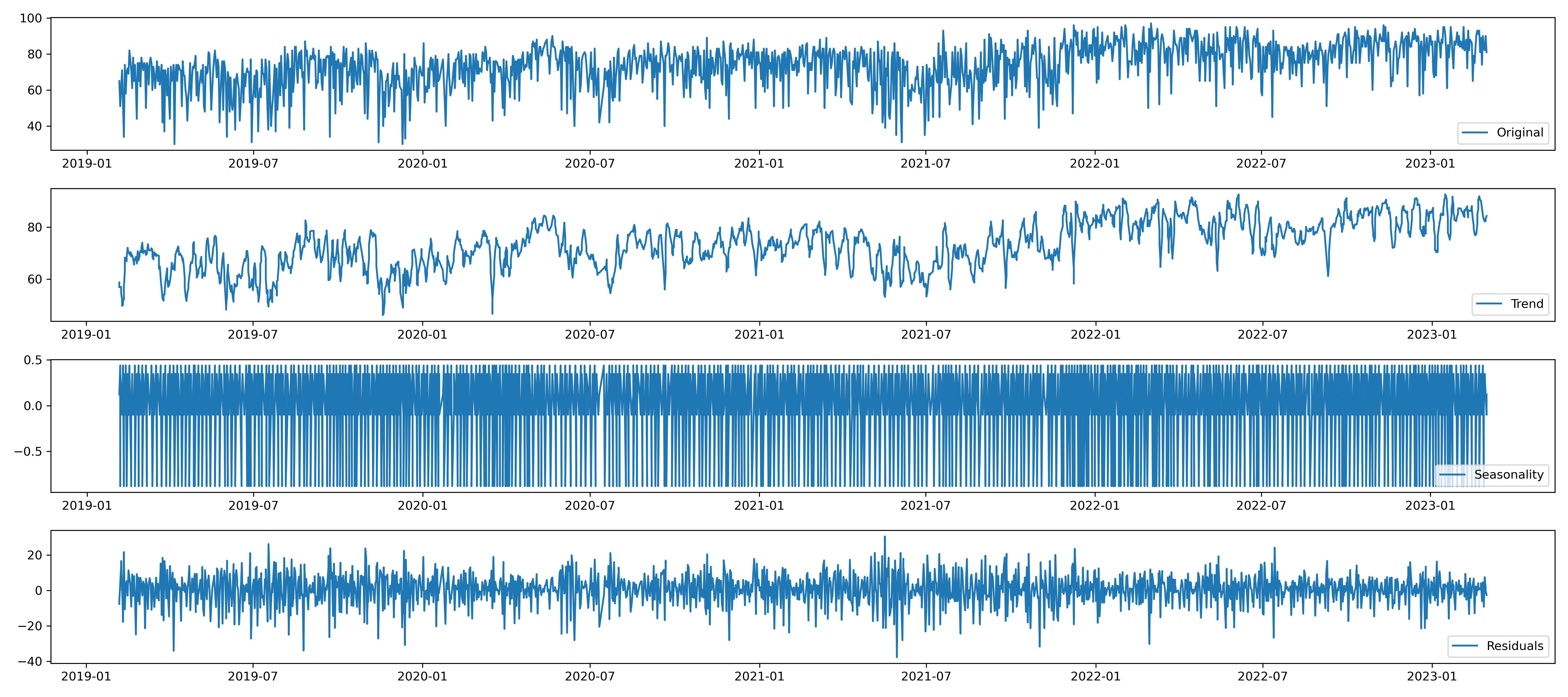
I visualized a time series decomposition to better understand the presence of trend in the sleep score dataset.

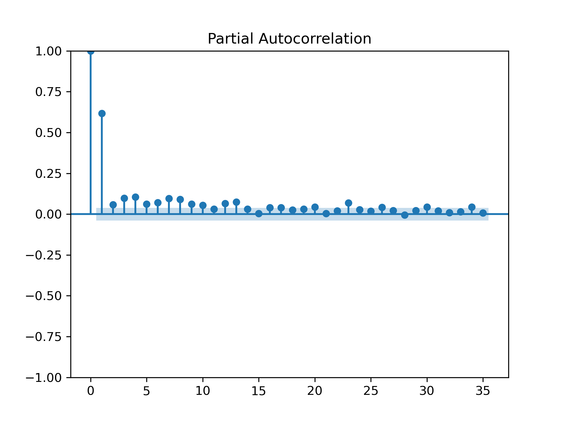
Additionally, I plotted a partial autocorrelation function using statsmodels. Notably, partial autocorrelation appears to drop to zero for lag values greater than 2.

Lag Order Selection

The number of lags amount to the number of preceding days included as predictor values in the model. The statsmodels function select_order() was used to assess an optimal lag value with possibilities between 0 and 15. The optimal lag value was determined using four information criteria — Akaike Information Criteria (AIC), Bayes Information Criterion (BIC), Final Prediction Error (FPE), and Hannan-Quinn (HQ) criterion. This selection process yielded a tie with lag-1 and lag-2 each labeled as the minimum on these criteria. In this case, I selected lag-2 based on prior knowledge of sleep quality and the onset of mood states.

	AIC	BIC	FPE	HQIC
0	1.688	1.708	5.408	1.695
1	-0.02482	0.09412*	0.9755	0.01979*
2	-0.03545*	0.1826	0.9652*	0.04635
3	-0.03417	0.2830	0.9664	0.08481
4	-0.02907	0.3872	0.9714	0.1271
5	-0.02537	0.4900	0.9750	0.1680
6	-0.01701	0.5975	0.9832	0.2135
7	-0.01940	0.6943	0.9809	0.2483
8	-0.01014	0.8026	0.9900	0.2948
9	-0.0008049	0.9111	0.9993	0.3413
10	0.01201	1.023	1.012	0.3913
11	0.02510	1.135	1.026	0.4415
12	0.03723	1.246	1.038	0.4909
13	0.04867	1.357	1.050	0.5395
14	0.06022	1.468	1.063	0.5882
15	0.07076	1.577	1.074	0.6359

Vector Autoregression Model

All time series under analysis were found to be stationary (ADF test $p$ < .05). The results of the VAR(2) model predicting mood states using sleep score are shown below. Sleep score was found to be a significant positive predictor of depression, also confirmed via Granger causation tests. Sleep score did not positively or negatively predict other mood states in this model.

	Coefficient	Std. error	Test statistic	p-value
L1.score	0.633262	0.027574	22.966	0.000
L1.anxious	0.153275	0.446110	0.344	0.731
L1.depressed	0.477164	0.409130	1.166	0.243
L1.irritable	-0.282988	0.412509	-0.686	0.493
L1.elevated	-0.220198	0.655784	-0.336	0.737
L2.score	-0.003080	0.027452	-0.112	0.911
L2.anxious	0.353528	0.445359	0.794	0.427
L2.depressed	1.241873	0.409667	3.031	0.002
L2.irritable	-0.080069	0.412341	-0.194	0.846
L2.elevated	-0.499540	0.657230	-0.760	0.447

Granger Causality

The results of the Granger causation tests are shown below. Sleep score was shown to Granger-cause both depressed and anxious mood.

Causal Variable	Variable	Test statistic	Critical value	p-value	df
sleepscore	depressed	5.384	2.997	0.005	(2, 6535)
sleepscore	anxious	3.294	2.997	0.037	(2, 6535)
sleepscore	irritable	1.347	2.997	0.260	(2, 6535)
sleepscore	elevated	1.203	2.997	0.500	(2, 6535)

Impulse Response Analysis

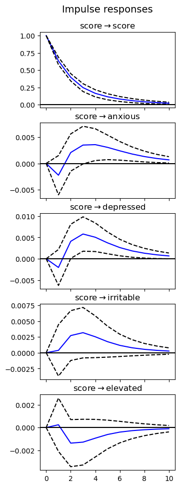
As shown in the figure below, the impact of sleep score on the four self-reported mood states varies over a 10-day period. Standard errors are plotted at the 95% significance level. The effect of an impact on sleep score on depressed and anxious moods appear to be most felt only after several days of its impact, peaking at roughly 3 days and then gradually decaying.

Discussion

This exploratory study affirms the role that self-tracking technologies can play in the ongoing management of affective disorders. This type of N-of-1 analysis would be impossible without inexpensive wearable sensors, and the quality of this dataset is directly related to how non-invasive this particular wearable is.

This work is limited in several ways. My reliance on an algorithmic ADF test to assess stationarity (rather than directly assessing the data myself) could leave room for error. Additionally, this work only assesses the influence of the Oura sleep score on mood. In reality, this is likely closer to a bidirectional influence and this should be reflected properly in the analysis.